Decision Tree

Decision Tree

A decision tree is a flowchart-like tree structure in which each internal node represents a split based on a feature condition while each leaf node represents a class label. And it is non-parametric supervised learning method which can be used for both classification and regression tasks. The difference between classification and regression in decision tree is that whether the predicted value in each leaf node is discrete set of values or continuous values (real numbers ).

Information Gain

Information Gain is used to determine which feature on which condition to split on at each step in building the tree. Our goal is to find a serious of split point so that each leaf contains the same label or pure label. The internal node contains mixed labels or has some impurity. When we want to split a node with mixed labels, we prefer to choose the feature on some condition so that the average impurity of two split node is less than the parent node, in other words, the children node label are much purer than its parent. Then we say based on this split we gain some information.

Qualitatively speaking,

Information Gain = Impurity(parent node) - Average of impurity(children node)

Assuming the number of data points at parent node is \(D_{parent}\), we split the data points into two children node based on a feature and the number of data points at left child node is \(D_{left\_child}\) and the number of data points at right child node is \(D_{right\_child}\), then

There are different ways to capture the impurity quantitatively and here we introduce two methods entropy and Gini impurity.

Entropy Impurity

Entropy is a common way to measure impurity.

If the dataset is pure in which all the data points have the same label, the entropy is 0. The higher impurity is, the higher entropy is. And the higher the entropy is, the more information the dataset content.

The information gain for one split or for one internal node is that

Information Gain = entropy(before split) - average entropy (children)

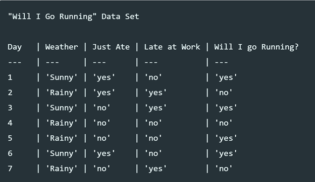
We use Fig.1 to show an example how to calculate the entropy of a node and the average entropy after splitting. Assuming the points in dataset belong to one node, it contains 3 “no” labels and 4 “yes” labels, so the entropy of this node is

Assuming we split based on “weather”, one child node contains all “Sunny” points (3 data points) and the other contains all “Rainy” points (4 data points). For the “Sunny” child node, the total number of data points is 3 with all “yes” labels, the entropy for this child is

For the “Rainy” child node, the total number of data points is 4 with 1 “yes” label and 3 “no” labels, the entropy for this child is

So the average entropy of children nodes is

The information gain based on entropy impurity is

There is a special case that the children data points labels distribution is exactly the same as parents then information gain is 0 which means we didn’t get any more information based on this split.

Gini Impurity

Gini impurity is another method to calculate the impurity. And its formula is

Same as entropy, when the dataset contains pure labels, Gini cost is 0.

Using the same dataset above, the Gini cost of the dataset is

Again, we split based on “Weather”, and the Gini cost for “Sunny” child node is

The Gini cost for “Rainy” child node is

Therefore, the information gain based on this split is

Comparison between Entropy and Gini

• When the dataset has the same label, both has value 0
• When the data points are evenly distributed among \(C\) different labels, both has a maximum value. The maximum value for entropy is \(-log_2\frac{1}{C}\) and the maximum value for Gini is \(1-\frac{1}{C}\).
• Neither metric result the more accurate tree than the other. A slight preference might go to Gini since it doesn’t involve a more computationally intensive log to calculate

Learning algorithm

Here shows a pseudo code:

# pseudo code
fitTree(D,depth):
    node = Node(D)
    if node is not worth splitting:
        return node
    else:
        choose the best feature and split condition with the most information gain
        node.left = fitTree(Node(D_left),D_left,depth+1)
        node.right = fitTree(Node(D_right),D_right,depth+1)
        return node

When node is not worth splitting:

• node is pure
• depth exceeds max depth (set by us)
• \(D\_left\) or \(D\_right\) is too small
• Information gain is too small

Note: this algorithm is a top-down, greedy approach, at each node splitting is based on local training examples

Issues in decision trees

The deeper the tree, the more complex the rules and fitter the model. Overfitting is big problem in decision tree.

Ensemble Methods

Ensembles combines multiple models to improve the prediction instead of using a single model.

Bagging (bootstrap aggregating)

Bagging trains each model in the ensemble using a randomly drawn subset of the training set. The results from each learner are combined in the form of voting.

Random forest

The random forest algorithm combines random decision trees with bagging to achieve very high classification accuracy and each decision trees is build on a subset drawn with replacement from the training set.

Boosting

Boosting involves incrementally building an ensemble by training each new model instance to emphasize the training instances that previous models misclassified. In some cases, boosting has been shown to yield better accuracy than bagging but it also tends to be more likely to overfit the training data.

AdaBoost

Gradient Tree Boosting

Reference:

• Prince Yadav. Decision Tree in Machine Learning
• Information Gain
• Brain Ambielli. Gini Impurity (With Examples)
• Avinash Navlani. Decision Tree Classification in Python
• https://www.hackerearth.com/practice/machine-learning/machine-learning-algorithms/ml-decision-tree/tutorial/
• Wikipedia. Ensemble learning